Constructing Pedigrees in R

I was looking for a good way to draw pedigrees using software, without having to fuss drawing them “by hand” using a drawing program. Lo and behold, I came across a few different packages in R that allow me to do just that!

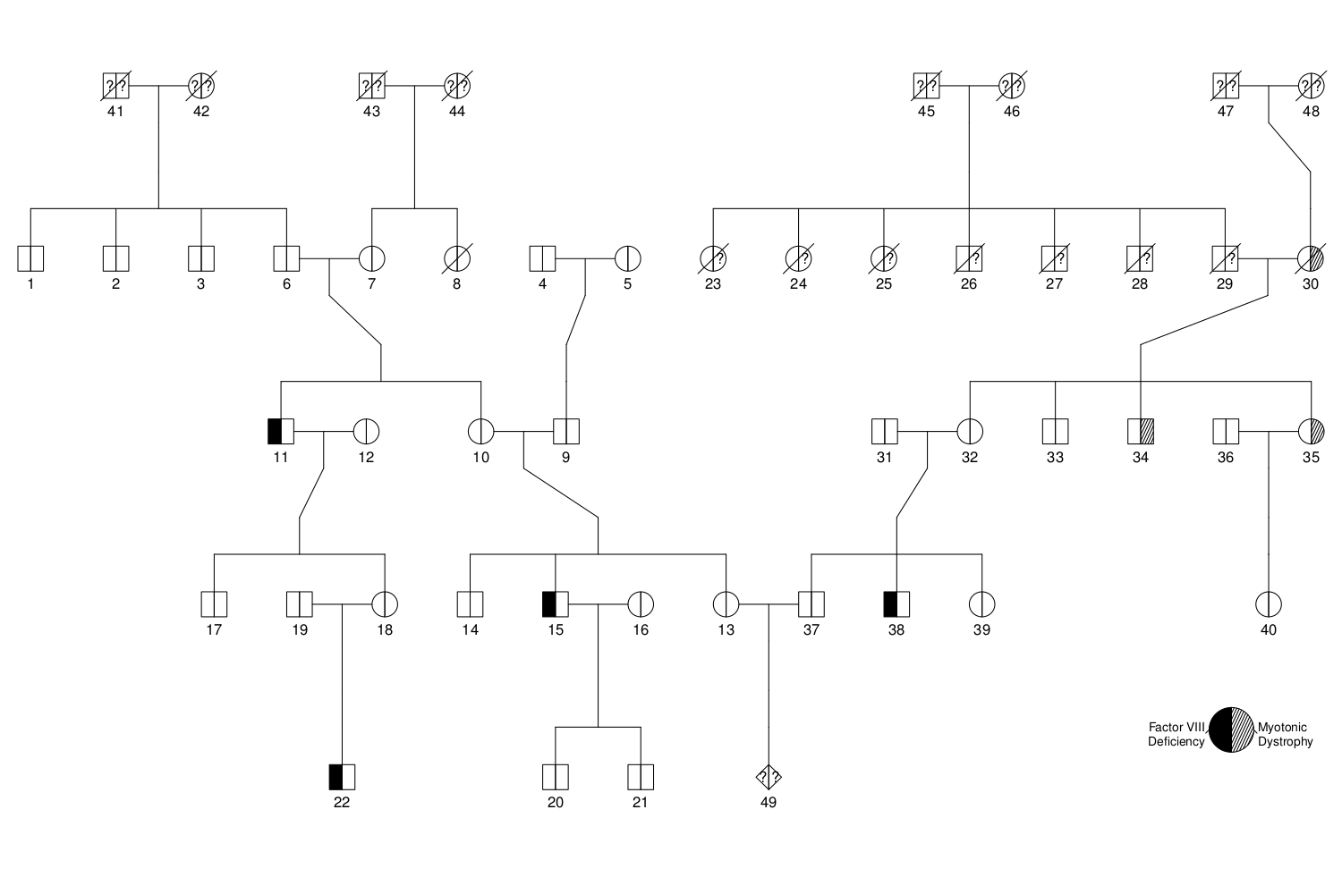
Using the kinship2 package, I was quickly able to produce a nice pedigree for a family with two genetic conditions: factor VIII deficiency (haemophilia) and myotonic dystrophy. Factor VIII deficiency is a classic example of a sex-linked recessive trait, and myotonic dystrophy follows autosomal dominant inheritance. In this pedigree, I show the status of affected and unaffected indiviudals (not carriers), using the following bits of code in R.

First, let’s install (if needed) and load the kinship2 package:

if (!require(kinship2)) {install.packages("kinship2"); library(kinship2)}

Now we need to code several variables which will correspond to all of the individuals in the pedigree. First, we need individual ID numbers:

ids <- 1:49

Second, we need to identify the father and mother of each individual using the individual ID numbers above:

dad <- c(41,41,41,NA,NA,41,43,43,4,6,6,NA,9,9,9,NA,11,11,NA,15,
		 15,19,45,45,45,45,45,45,45,47,NA,29,29,29,29,NA,31,31,31,36,
		 NA,NA,NA,NA,NA,NA,NA,NA,37)
mom <- c(42,42,42,NA,NA,42,44,44,5,7,7,NA,10,10,10,NA,12,12,NA,16,
		 16,18,46,46,46,46,46,46,46,48,NA,30,30,30,30,NA,32,32,32,35,
		 NA,NA,NA,NA,NA,NA,NA,NA,13)

Now we code the sex and status (0=alive, 1=dead) of each individual:

sexes <- c(1,1,1,1,2,1,2,2,1,2,1,2,2,1,1,2,1,2,1,1,1,1,2,2,2,1,1,1,1,
		   2,1,2,1,1,2,1,1,1,2,2,1,2,1,2,1,2,1,2,3)
dead <- c(0,0,0,0,0,0,0,1,0,0,0,0,0,0,0,0,0,0,0,0,0,0,1,1,1,1,1,1,1,1,
		  0,0,0,0,0,0,0,0,0,0,1,1,1,1,1,1,1,1,0)

Here is where we code the affected status of each individual (0=unaffected, 1=affected, NA=unknown). We need to bind these columns together in a matrix (you can have up to 4 traits; one per column):

F8 <- c(0,0,0,0,0,0,0,0,0,0,1,0,0,0,1,0,0,0,0,0,0,1,0,0,0,0,0,0,0,0,
		0,0,0,0,0,0,0,1,0,0,NA,NA,NA,NA,NA,NA,NA,NA,NA)
MD <- c(0,0,0,0,0,0,0,0,0,0,0,0,0,0,0,0,0,0,0,0,0,0,NA,NA,NA,NA,NA,NA,NA,1,
		0,0,0,1,1,0,0,0,0,0,NA,NA,NA,NA,NA,NA,NA,NA,NA)
affect <- as.matrix(cbind(F8, MD))

And now we create the pedigree object and plot it:

family <- pedigree(id=ids, dadid=dad, momid=mom,
				   affected=affect, sex=sexes, status=dead)

plot.pedigree(family)

pedigree.legend(family, location="bottomright",
				labels=list("Factor VIII\nDeficiency", "Myotonic\nDystrophy"),
				cex=0.8, radius=0.3)

That’s the basics! Of course, with a large pedigree I expect this becomes a bit unruly, but for smaller examples like this one it’s relatively easy to put together.